TOPICS

Editor Essentials Scripting Graphics & Visual Effects 2D Mobile & Touch XR Physics User Interface For Educators AI & Navigation

Content Type

Pathways

Build skills in Unity with guided learning pathways designed to help anyone interested in pursuing a career in gaming and the Real Time 3D Industry.

View all Pathways

Courses

Explore a topic in-depth through a combination of step-by-step tutorials and projects.

View all Courses

Projects

Create a Unity application, with opportunities to mod and experiment.

View all Projects

Tutorials

Find what you’re looking for with short, bite-sized tutorials.

TOPICS

View Tutorial Content

Creating a Vertex Displacement Shader

Tutorial

Intermediate

+0 XP

20 Mins

(47)

Summary

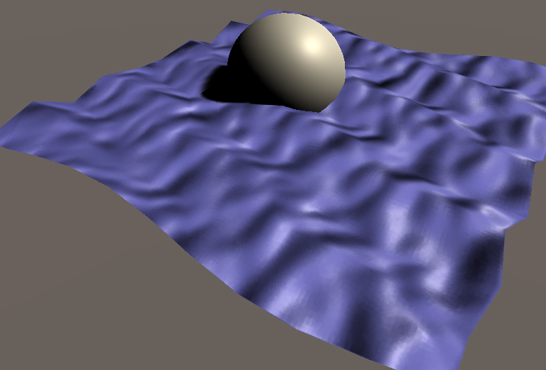
In this tutorial, we will use Unity’s default render pipeline to create a shader that will deform and animate a flat mesh over time to simulate the motion of an ocean’s surface. 

Select your Unity version

Last updated: June 26, 2023

2019.4

Language

English

Creating a Vertex Displacement Shader